Measuring soil resistivity is essential before designing a grounded earthing system for a substation. Because this measurement determines how well the ground can dissipate fault currents. If the soil resistivity is high, the grounding system needs some changes. It requires denser earthing mesh and more conductive electrodes. A well-designed earthing system prevents intolerable voltage buildup. Obviously, the well-designed earthing system protects equipment and reduces the risk of electric shock. Since soil resistivity varies with depth, moisture, and composition. Accurate testing helps in selecting the right grounding method. Poor measurement can cause the grounding system to fail. This leads to dangerous faults.
Wenner Method of Soil Resistivity Measurement
The Wenner four-electrode method is the most popular for earth resistivity measurement. It gives accurate and reliable results. The setup is also simple. The Wenner method uses four equally spaced electrodes. We adjust the spacing between electrodes for different readings. Wider spacing measures deeper soil layers. Obviously, this is useful for understanding different soil layers. It also reduces errors caused by contact resistance. The Wenner method shows how resistivity varies across the soil.
In the Wenner method, we insert four electrodes in a straight line on the ground. We place the electrodes in an equal gap. The outer two electrodes inject a constant electric current into the ground. At the same time, the inner two electrodes measure the voltage drop. At the same time, the inner two electrodes measure the voltage drop caused by this current.

The soil resistivity is then calculated using the formula\[\rho = 2\pi\times a \times R \] Where \(a\) is the spacing between the electrodes and \(R\) is the measured resistance.
Details Method Step by Step
First, we insert the metal rods (electrodes) into the ground at a fixed distance. We do it along a straight line. Then we place a ground resistance meter at the center of the line, as shown. Then we connect the meter to these electrodes using cables. The meter injects a known current through the outer electrodes \(C_1 and C_2\). The inner electrodes \(P_1 and P_2\) measure the resulting voltage drop.
Then, we change the location of the electrodes along the same straight line. Now, we repeat the test with this new value of spacing \(a\). We can test deeper soil by spacing electrodes farther apart. No digging is needed. In this way, we repeat the test for different spacings along the same straight line. As per standards, these spacings are \{\text{a = 2m, 5m, 10m, 15m, 25m, 50m \cdot\cdot\cdot}\]
Spacing can go up to 250m. This depends on the measurement area and other conditions.
We must repeat the measurement in different directions. Keep the meter at the same central location. As per normal practice, we use north-south, east-west, and their diagonal directions.
If the ground is too dry or rocky, adding water or using conductive gel can help improve contact. Environmental factors like soil moisture and temperature can also affect results. Therefore, test under different conditions. This gives reliable data. We must avoid testing in rainy seasons. Because wet soil gives misleading results.
Practical Example of Using the Wenner Method
Let us conduct the Wenner method of soil resistivity for a substation site. For that, we must follow standard practices. First, we locate the reference point of measurement. The location must be such that the maximum area of the substation comes under the test zone. Then we consider the north-south direction. After that, analog north-south straight line, we place the electrodes considering the spacing \(a = 2 m\). The depth of the electrodes should not exceed 1/20th of the spacing between them (\a\). Now, we connect the electrodes to the resistance meter using test leads.

Then, we set the meter to the soil resistivity measurement mode. As a result, it injects a known current to the soil through C1. The current then returns through C2. The meter measures the voltage drop between P1 and P2. Then the meter displays the ratio of the measured voltage and the injected current i.e. resistance (R). Using the formula \(\rho = 2\pi aR\), calculate the soil resistivity \((\Omega – ·m)\).
Repeat of Measurements
Now, we repeat the measurement and associated resistivity calculation by relocating the spikes at other standard spacings like 5m, 10 m, 15m, etc., along the same straight line. After that, we repeat the measurements in different directions (North-South, East-West, Northeast-Southwest, and Northwest-Southeast) to account for soil non-uniformity.
At last, from all the resistivity values we have to calculate the overall soil resistivity. This is the test for one point or location.
Relation between Electrode Spacings and the Depth of the Soil being measured for Resistance
Here, the spacing between the electrodes (a) directly affects how deep the measurement goes. The injected current spreads out in a semi-spherical pattern. So, the larger the spacing, the deeper the current penetrates. Hence, it samples more soil layers. Therefore, the electrode spacing (a) determines the approximate depth of soil being measured. Simply put:
- If the electrodes are 2 meters apart, the resistivity measurement represents the soil down to about 2 meters.
- If the spacing increases to 5 meters, the reading reflects an average resistivity down to around 5 meters.
To analyze resistivity at different depths, we step by step increase electrode spacing (e.g., 2m, 5m, 10m, 15m, etc.). The calculated final reading gives a weighted average rather than a precise layer-by-layer breakdown. For more accuracy, additional interpretation techniques (like computer modeling) help separate the influence of shallower layers from deeper ones. The computer modeling uses a polar curve to determine overall soil resistivity.
In short, increasing electrode spacing in the Wenner Method lets you measure deeper soil resistivity, but the result is an average over that depth rather than a direct measurement of the deepest point.
Calculating Overall Soil Resistivity
Sometimes, the average resistivity values in different directions are not similar. While this difference becomes more than 20 to 30%, we use the polar curve method to calculate the overall soil resistivity of that location. In such cases, the simple average of the calculated resistivity values in all directions cannot represent the actual or approximate resistivity of the soil. Here, we use the polar curve method. Here, we plot the calculated average resistivity on the axis of each measuring direction. Each point is placed at a distance from the center. That distance corresponds to the average resistivity value calculated for that direction.
In this way, we plot the resistivity values along north, northeast, east, southeast, south, southwest, west, and northwest directions. We then join all the plotted points, representing the resistivity values in their respective directions, using straight lines to form a closed curve.
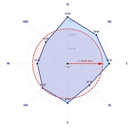
Next, we calculate the area enclosed by this closed polar curve. After that, we draw a circle having the same area as that covered by the polar curve. The radius of this circle gives the equivalent soil resistivity of that location.
Video on Polar Curve Method with Wenner Four Electrode Method