The vector diagram shows the phase relationships clearly. It reveals how currents and voltages interact physically. Moreover, it guides us in circuit element placement. Each vector represents one specific circuit component. Therefore, the diagram becomes our blueprint for the equivalent circuit of a transformer. Without it, we cannot understand parameter connections properly.
Vector Diagram
No Load Current
Let me explain this step by step clearly.
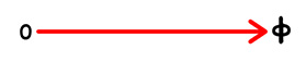
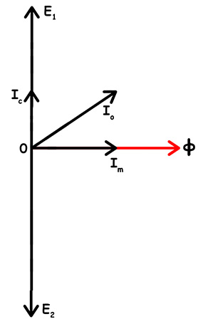
Magnetic Flux: First, we take the magnetic flux \(\phi\) as a reference. The flux lies along the horizontal axis. This flux links both primary and secondary windings.
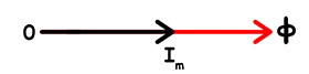
Magnetizing Current: The magnetizing current \(I_m\) creates the flux. Therefore, \(I_m\) is in phase with \(\phi\). Consequently, \(I_m\) also lies on the horizontal axis. This current magnetizes the transformer core.
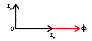
Core Loss Current: The core has losses due to hysteresis. Additionally, eddy currents cause more losses. The core loss current \(I_c\) supplies these losses. These losses appear as heat in the transformer core. Importantly, \(I_c\) leads the flux by 90°. Thus, \(I_c\) lies along the vertical axis. This represents the loss component clearly.
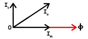
No-Load Current: Now, we combine \(I_m\) and \(I_c\) vectorially. The no-load current \(I_o\) is their vector sum. Therefore: \[ I_o = I_c + I_m \text{(vector addition)}\] \(I_o\) lags behind the applied voltage \(V_1\). The angle is typically 70° to 80°. This current flows when the secondary is open.
Induced EMFs in the Windings
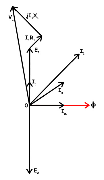
The changing flux induces EMF in windings. \(E_1\) is induced in the primary winding. Similarly, \(E_2\) is induced in the secondary winding. Both \(E_1\) and \(E_2\) oppose the flux. Hence, they lag the flux by 90°. They point downward on the vertical axis.
Primary Applied Voltage
\(V_1\) is the applied primary voltage. \(V_1\) must overcome several voltage drops. First, it drops across primary resistance \(R_1\). The drop is \(R_1I_1\) in phase with \(I_1\). Next, it drops across leakage reactance \(X_1\). The drop is \(X_1I_1\) leading \(I_1\) by 90°. Finally, \(V_1\) must balance \(E_1\). Therefore: \[V_1 = E_1 + I_1R_1 + jI_1X_1\]
Secondary Load Voltage
When the load connects, current flows in the secondary. \(I_2\) flows through the secondary winding. \(E_2\) is the induced secondary voltage. However, \(V_2\) appears across the load terminals. \(V_2\) is less than \(E_2\) due to drops. The secondary resistance \(R_2\) causes \(I_2R_2\) drop. The leakage reactance \(X_2\) causes \(I_2X_2\) drop. Therefore: \[V_2 = E_2 – I_2R_2 – jI_2X_2\]
Actual Primary Current: Secondary current \(I_2\) creates a demagnetizing effect. Consequently, primary draws more current to compensate. Let\({I_2}’\) be \(I_2\) referred to the primary. Then, \[{I_2}’ = I_2\frac{N_2}{N_1}\]
The actual primary current \(I_1\) has two components. First component is \(I_o\) (the no-load current). The second component is \({I_2}’\) (the load component). Thus: \[I_1 = I_o + {I_2}’\text{(vector sum)}\]This, \({I_2}’\) is nearly opposite to \(I_2\) direction. Let me now draw the complete vector diagram of transformer.
Equivalent Circuit of Transformer
Now, let’s convert this diagram into a circuit.
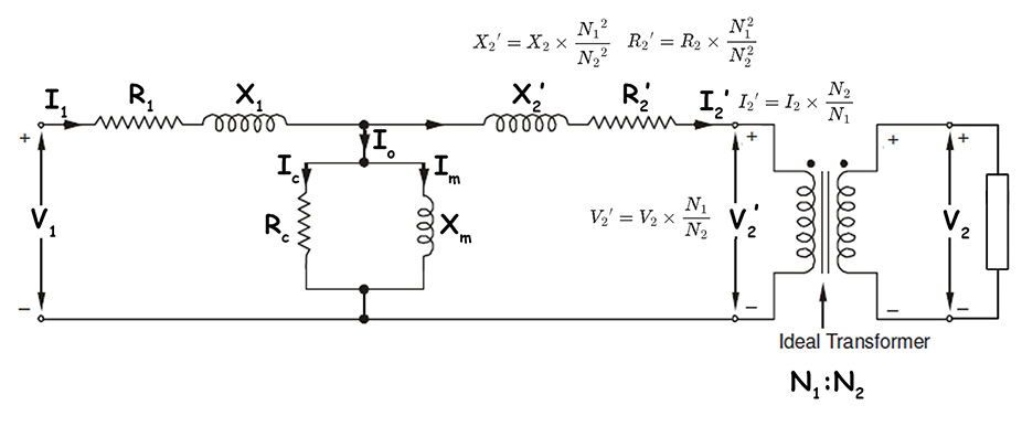
Representing the Core Loss: \(I_c\) represents the core loss component. We model this using a resistance \(R_c\). \(R_c\) connects in parallel with the winding. We can represent the core power loss as \({I_c}^2R_c\text{ watts}\). Such as \(I_c\) flows through \(R_c\).
Representing the Magnetizing Current: \(I_m\) represents the magnetizing current. We model this using a reactance \(X_m\). \(X_m\) also connects in parallel with \(R_c\). Together, \(R_c\) and \(X_m\) form the excitation branch. Since, the No-Load current \(I_o\) is the sum of \(I_c\) and \(I_m\), we represent \(R_c\) and \(X_m\) in parallel combination. This branch connects across the primary winding.
Primary Resistance and Leakage Reactance
\(I_1R_1\) drop requires series resistance \(R_1\). Similarly, \(I_1X_1\) drop requires series reactance \(X_1\). Both \(R_1\) and \(X_1\) connect in series. They appear before the excitation branch.
The Ideal Transformer
Between primary and secondary, an ideal transformer exists. Its turns ratio is \(N_1:N_2\). It transforms voltage as \(E_2 = E_1\frac{N_2}{N_1}\). Similarly, it transforms current as \({I_2}’ = I_2\frac{N_2}{N_1}\).
Secondary Resistance and Leakage Reactance
\(I_2R_2\) drop requires series resistance \(R_2\). \(I_2X_2\) drop requires series reactance \(X_2\). Both connect in series on the secondary side. They appear after the ideal transformer. Finally, we come to the load. Load voltage \(V_2\) appears across load terminals. Load current \(I_2\) flows through the load.
Equivalent Circuit of Transformer Referring to Primary Side
A transformer has two separate windings physically. Primary has its own resistance and reactance. Similarly, secondary has its own resistance and reactance. Therefore, analyzing both sides separately becomes complex.
When we view from the primary side, we ask
- What equivalent resistance of primary would cause the same copper loss as the secondary?
- What equivalent reactance of the primary would store the same magnetic energy as the secondary?
These equivalent values become the referred parameters.
Secondary Resistance Referred to Primary
Secondary copper loss is \(I_2^2R_2\) watts. This heat dissipates in the secondary winding. Now, we want an equivalent resistance on the primary side that causes the same loss. The transformation ratio is \(\frac{N_2}{N_1}\). Secondary current \(I_2\) transforms to the primary side is \[{I_2}’ = I_2 \times \frac{N_2}{N_1}\]For the same power loss on the primary side\[{{I_2}’}^2{R_2}’ = {I_2}^2R_2\] \[\text{Substituting}{I_2}’ = I_2 \times \frac{N_2}{N_1}\]\[\left[I_2 \times \frac{N_2}{N_1}\right]^2 {R_2}’ = I_2^2R_2\]\[I_2^2 \times \frac{N_2^2}{N_1^2} \times {R_2}’ = I_2^2R_2\]\[\text{Canceling} (I_2^2) \text{from both sides}\]\[\frac{N_2^2}{N_1^2} \times {R_2}’ = R_2\]Therefore, we get\[{R_2}’ = R_2 \times \frac{N_1^2}{N_2^2}\]This ensures identical power loss!
It’s an imaginary resistance on the primary side. This resistance doesn’t physically exist there. However, it produces the same power loss as secondary. In other words, the loss equals the actual secondary copper loss.
Energy Stored in Secondary Reactance
Similarly, magnetic energy is stored in secondary reactance. The energy stored is proportional to \(I_2^2X_2\). Following the same mathematical process\[{X_2}’ = X_2 \times \frac{{N_1}^2}{{N_2}^2}\]This ensures identical energy storage!
It’s an imaginary reactance on the primary side. Obviously, this reactance doesn’t physically exist there. However, it deals the same magnetic energy. Actually, this energy equals the actual secondary leakage flux energy.
Voltage Transformation
Secondary voltage also needs transformation. The voltage transformation ratio is \(\frac{N_1}{N_2}\). Therefore\[{V_2}’ = V_2 \times \frac{N_1}{N_2}\]
Referring Transformer Circuit to Secondary Side
Previously, we referred everything to the primary side. However, we can do the opposite, too. We can refer everything to the secondary side instead. This approach is equally valid and useful. The choice depends on our analysis requirements.
The fundamental principle remains identical. When viewing from the secondary side.
- What equivalent resistance of secondary would cause the same copper loss as the primary?
- What equivalent reactance of the secondary would store the same magnetic energy as the primary?
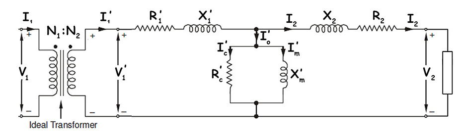
Primary current \(I_1\) flows through primary winding. When referred to secondary, it becomes \({I_1}’\). The turns ratio determines this transformation. However, now the ratio is inverted. Therefore\[{I_1}’ = I_1 \times \frac{N_1}{N_2}\]Notice: This is opposite to the primary reference. This is how primary current appears from secondary.
Equivalent Primary Resistance Referred to Secondary
Now, copper loss occurs in \(R_1\). The actual loss is \({I_1}^2R_1\) watts. This heat dissipates in the primary winding.
What equivalent secondary-side resistance represents this? Let’s call this equivalent resistance \({R_1}’\). The referred current \({I_1}’\) flows through \({R_1}’\). Therefore, loss in \({R_1}’\) is \({{I_1}’}^2{{R_1}’}\). For equivalence, these losses must be equal\[{{I_1}’}^2{R_1}’ = {I_1}^2{R_1}\]Now, substitute \[{I_1}’ = I_1\frac{N_1}{N_2}\]\[\left[I_1 \times \frac{N_1}{N_2}\right]^2{R_1}’ = {I_1}^2R_1\]Expanding the square\[{I_1}^2 \times \frac{{N_1}^2}{{N_2}^2} \times {R_1}’ = {I_1}^2R_1\]Cancel \({I_1}^2\) from both sides\[\frac{{N_1}^2}{{N_2}^2} \times {R_1}’ = R_1\]Therefore, solving for \({R_1}’\)\[{R_1}’ = R_1 \times \frac{{N_2}^2}{{N_1}^2}\]This \({R_1}’\) causes identical power loss!
Equivalent Primary Reactance Referred to Secondary
Similarly, magnetic energy is stored in \(X_1\). The stored energy is proportional to \({I_1}^2X_1\). Again, we need an equivalent reactance \({X_1}’\). Following the same mathematical process,\[{X_1}’ = X_1 \times \frac{{N_2}^2}{{N_1}^2}\] This \({{X_1}’}\) stores identical magnetic energy!
Voltage Transformation
Primary voltage also needs transformation. The voltage transformation follows the turns ratio inversely. Therefore\[{V_1}’ = V_1 \times \frac{N_2}{N_1}\]
Excitation Branch Transformation
The excitation branch also needs transformation. The core loss resistance \(R_c\) transforms as\[{R_c}’ = R_c \times \frac{N_2^2}{N_1^2}\]Magnetizing reactance \(X_m\) transforms as\[{X_m}’ = X_m \times \frac{{N_2}^2}{{N_1}^2}\]However, often we keep these on primary side. This is because they naturally connect across primary.
Verification of Power Conservation
Let’s verify that power remains unchanged.
Actual primary power\[P_1 = V_1 \times I_1 \times \cos\phi\]Referred primary power\[P_1′ = V_1′ \times I_1′ \times \cos\phi\]Substitute the transformed values\[{P_1}’ = \left(V_1 \times \frac{N_2}{N_1}\right) \times \left(I_1 \times \frac{N_1}{N_2}\right) \times \cos\phi\]The fractions cancel out\[P_1′ = V_1 \times I_1 \times \cos\phi\]Therefore\[{P_1}’ = P_1\]Power is perfectly conserved!