Before entering the article on the transformer vector diagram or the transformer phasor diagram, we may recall our concept of an ideal transformer. For a basic idea of an ideal transformer, you may also read our article on the emf equation of a transformer.
Considering Core Losses for Transformer Vector Diagram
Now, we shall consider the core losses of a transformer. Suppose this transformer is in a no-load condition. The primary input current under no-load conditions has to supply the iron loss in the core. Iron loss is the sum of hysteresis loss and eddy current loss. A very small amount of copper loss also occurs in the primary winding. This happens because the no-load current has to flow through the primary winding. However, we normally neglect this ohmic loss. Because of core losses, the no-load primary input current does not exactly lag 90° behind \( V_1 \), rather it lags it by an angle less than 90°. Say, this angle is \(\theta_0\).
No-load primary input power will be \[ \boldsymbol{W_o = V_1 I_o \cos \theta_o }\] No load primary current \( I_o \) has two components. One in phase with \( V_1 \). Obviously, this is the active component or working component or iron loss component \( I_w \). It supplies the iron loss and the neglected small quantity of primary copper loss. \[ \boldsymbol{I_w = I_o \cos \theta_o} \] Other one is in quadrature with \( V_1 \).
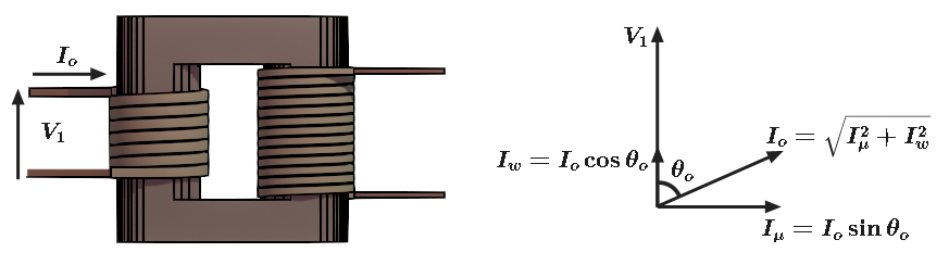
We refer to it as the magnetizing component \( I_{\mu} \). This component of no load current sustains the alternating flux in the core. So, it is wattless. \[\boldsymbol{ I_{\mu} = I_o \sin \theta_o }\] Thus, \( I_o \) is the vector sum of \( I_o \) and \( I_{\mu} \) \[ \boldsymbol{ I_o = \sqrt{I_{\mu}^2 + I_w^2}} \]The no-load current is quite small compared to the full-load current of a transformer.
Considering Connected Secondary Load for the Transformer Vector Diagram
Now we connect the secondary with a load. Here, the load is a resistor as shown in the above image. The secondary current \( I_2 \) starts flowing. The secondary current contributes its own mmf (\(I_2N_2\)). Because of this mmf the secondary winding creates its own flux \(\phi_2\). This flux is in opposition to the main primary \(\phi\). The opposite secondary flux \(\phi_2\) weakens the primary flux momentarily. Hence, the primary back emf \( E_1 \) tends to reduce. For a moment, \( V_1 \) gains the upper hand over \( E_1 \). This causes more current \( I_1′ \) to flow in the primary.
This current is known as the load component of primary current. This current is in phase opposition to current . Therefore, the primary mmf sets up a flux which opposes . Obviously, is in the same direction as . It is needless to say, . Thus, the magnetic effect of secondary current gets neutralized immediately by additional primary current . Hence, whatever the load conditions, the net flux remains constant.
Hence, the total primary current from the source is
Considering Winding Resistance for the Transformer Vector Diagram
An ideal transformer has no resistance. But in reality, a transformer has resistance in its windings. In other words, the primary and secondary windings have some resistance. Because of this resistance, there is a voltage drop in the windings.
If we consider that there is only pure resistance in the primary and secondary winding, there will be only a voltage drop on both the primary and secondary sides of the transformer. The secondary terminal voltage \( V_2 \) is equal to the vector difference of the secondary induced emf \( E_2 \) and the voltage drop across the secondary winding resistance \( I_2 R_2\). Moreover, the direction of this voltage drop will be along the direction of secondary current \( I_2 \). \[ \boldsymbol{V_2 = E_2 – I_2 R_2} \]
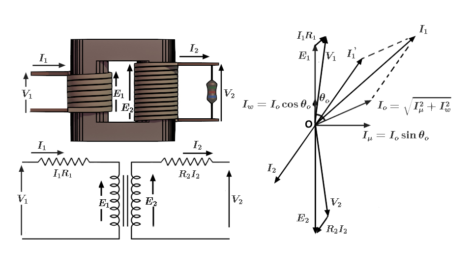
We get the primary induced emf \( E_1 \) from the vector difference between the source voltage \( V_1 \) and the voltage drop across the primary winding resistance \( I_1 R_1\). Obviously, the direction of this voltage drop will be along the direction of total primary current \( I_1 \). Additionally, the current \( I_1 \) is the vector sum of transforming current and no load current \( I_o \). Therefore, the transforming current refers to that current which is actually transformed to secondary. \[ \boldsymbol{E_1 = V_1 – {I_1} R_1} \]
Considering Winding Reactance for the Transformer Vector Diagram
In an ideal transformer, all the flux links both the primary and secondary windings. But in real transformers, this is not fully possible. Most of the flux links both windings, but some flux does not. So, we call it leakage flux. Hence, the leakage flux does not help in transferring energy between the windings.
On account of the leakage flux, both the primary and secondary windings have leakage reactance. Therefore, both windings will have self-induced emf. Obviously, the magnitude of the emf is a small fraction of the rated voltage. The primary terminal voltage \( V_1 \) therefore, has a component \( I_1X_1 \). As this is a pure reactance, the primary current \( I_1 \) lags the leakage reactance emf by 90o. Similarly, the secondary winding develops an emf of self-induction \( I_2X_2 \). Similarly, the secondary current \( I_2 \) lags the secondary leakage reactance emf by 90o.
Considering Both Winding Resistance and Reactance
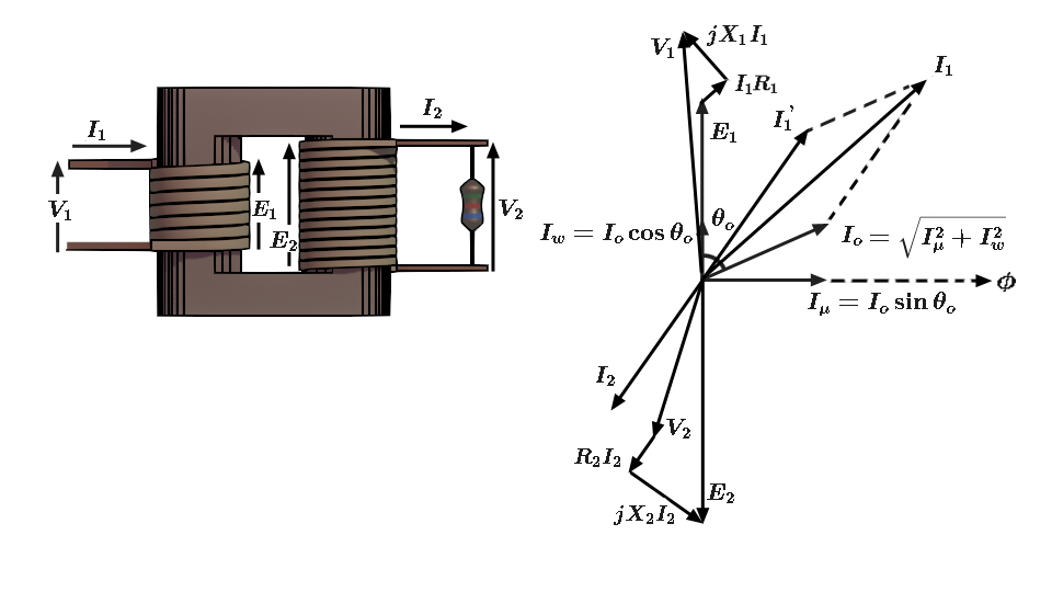
The primary impedance considering winding resistance and leakage reactance is given by\[ Z_1 = \sqrt{R_1^2 + X_1^2} \]Similarly, the secondary impedance considering winding resistance and leakage reactance is given by\[ Z_2 = \sqrt{R_2^2 + X_2^2} \]Therefore,\[V_1 = E_1 + I_1 (R_1 + jX_1) \]\[= E_1 + R_1I_1 + jX_1I_1 = E_1 + I_1 Z_1 \] \[ E_2 = V_2 + I_2 (R_2 + jX_2)\]\[ = V_2 + R_2I_2 + jX_2I_2 = V_2 + I_2 Z_2 \]