Definition of Transformer
A transformer is a static electrical device that transfers electrical energy from one circuit to another without changing the frequency.
Faraday’s Law of Electromagnetic Induction
Let us recall our knowledge of Faraday’s Law of Electromagnetic Induction. Because it is essential for the working principle of a transformer. This famous law states that when a changing flux links with a conductor, it induces a voltage across the conductor, and the value of this voltage is directly proportional to the rate of change of flux linkage with respect to time.
Now, we shall examine how, from this basic law of induction, we can develop a transformer.
Flux Linkage Between Two Coils
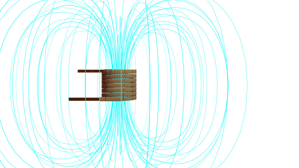
Let’s take a coil and supply it with an alternating source. We know that when a current flows through a coil, a magnetic field is developed in and around the coil. Naturally, flux will also be developed in and around the coil, as shown. This flux is also alternating, as the current through the coil is alternating. If the current from the source varies with a sinusoidal wave, the flux in and around the coil also varies sinusoidally.
Now, consider another coil nearby. This changing flux will link with the second coil. Therefore, according to Faraday’s Law of Electromagnetic Induction, a voltage—or better to say, an emf—is developed across the second coil. If we close the circuit connected to the second coil, a current starts flowing through it. So, we can conclude that this arrangement can transfer a portion of energy from the source to the second coil circuit without any direct electrical connection. This is the most basic working principle of a transformer.
Basic Structure of a Transformer
Now, we shall develop a basic transformer from this setup for better understanding. Here, you observed that the second coil links with only a small portion of the flux generated by the first coil. Hence, this arrangement transfers only a small portion of source energy.
If we need to transfer the entire energy supplied to the first coil, we need to link the entire flux with the second coil. For that, we obviously need to place a low-reluctance path between the first and second coils. We do this by using a closed core made of magnetic material like steel. Both coils surround the core. As soon as we place the core, it confines the entire flux within it. Therefore, the entire flux fully links with the second coil.
Basic Working Principle of a Transformer
In a simple transformer, we refer to the first coil as the primary winding and the second coil as the secondary winding. Now, we connect an alternating source across the primary winding. An alternating current starts flowing through the primary winding. Consequently, it develops a changing flux in the iron core. This flux is in phase with the input current.
Now, as per Faraday’s Law of Electromagnetic Induction, the emf induced in each conductor of the secondary winding varies directly with the rate of change of flux linkage. If there are \(N_2\) turns in the secondary winding, the total induced emf across the winding will be \(N_2\) times the emf per turn. If we express the flux with a sinusoidal wave, the emf will be a cosine wave, as this is the derivative of the flux function. So, this emf will lag the flux by 90 degrees.
Induction of Voltages in a Transformer
We can observe that the same flux links with the primary winding, too. Therefore, it induces the same emf per turn in the primary winding. Since the same changing flux links both windings, the same rate of change of flux applies to both. Now, say the number of turns in the primary winding is \(N_1\). Hence, the total induced emf across it will be \(N_1\) times the emf per turn.
As we have connected the source across the primary winding, according to Kirchhoff’s Voltage Law, the induced emf is equal and opposite to the source voltage. Here, the source voltage and induced primary voltage are equal and opposite. Therefore, ideally, the primary coil does not draw any current from the source. However, to maintain magnetization, the winding takes a small current. We refer to this small current as the magnetizing current.
Formation of Secondary Current
Until now, we have not connected any load across the secondary winding. If we now connect a load, as there is already an induced voltage across the secondary winding, a current starts flowing through the load as well as the secondary winding. We call this current as the secondary current. Obviousely, this current develops another flux in the core. This flux opposes the main magnetic flux. This means it will try to reduce the main magnetic flux.
But if the main flux decreases, the magnetic balance of the system will be disturbed. Therefore, the system tries to keep the magnetic flux constant. To do so, the system has to cancel out the additional flux generated by the secondary. This is done by drawing extra current from the source. The primary winding draws extra current to produce a counterflux that cancels the secondary flux. Thus, the net flux in the core remains constant—only the magnetizing flux.
Voltage and Current Relationship of a Transformer
The flux produced by a coil is directly proportional to the number of turns and the current in the coil. Since the primary and secondary fluxes are equal, the primary and secondary currents are inversely proportional to the number of turns. Also, the induced voltage across a winding is directly proportional to the number of turns. From these two relationships, we can conclude that the product of current and voltage for both windings is ideally the same. That also means, ideally, the power taken from the source is delivered to the load.
Step Up and Step Down Transformer
This simple system, consisting of two windings linked by a magnetic core, is the most basic model of a transformer. Here, you see that for a certain power output, both voltage and current in the secondary circuit depend on the number of turns in the secondary winding. If the number of turns in the secondary is greater than in the primary, the output voltage is greater than the source voltage, and the secondary current is less than the source current. This is called a step-up transformer. If the number of turns in the secondary is less, the output voltage is lower, and the current is higher. This is called a step-down transformer.
So, finally, we can say: a transformer is a static machine that transfers electrical power from the source circuit to the load circuit without changing the frequency, though the voltage and current levels may differ.